Abstract

Designing a controller for a real-world dynamical system is a challenge, particularly when the system is unknown, complex, chaotic, or nonlinear. A traditional project of a controller for such a system entails exhaustive data gathering for system identification or reinforcement learning (RL) training, often consuming significant time resources and potentially posing risks to the integrity of the system. In response to these challenges, we propose a method to completely virtualise a control system project from the real world that requires minimum knowledge of the underlying dynamical system and shows performance equivalent to real-world simulation-based methods. Central to our approach is the concept of the digital twin—a computational replica of the underlying system—which allows for the efficient and effective creation, testing, and validation the controller. This method can be applied to unknown complex dynamical systems where the controller is based on AI methods. Notably, our approach offers advantages over traditional RL techniques, boasting significantly reduced training time, heightened sample efficiency, and minimal reliance on hyperparameter fine-tuning. Finally, through experimental and numerical tests we demonstrate that our approach based on a model-free Next Generation Reservoir Computing (NGRC)¹ controller is capable of controlling highly complex, chaotic, nonlinear dynamical systems.

Table of contents

• Introduction
  • Background of reservoir computing and NGRC
    • How does reservoir computing work?
  • NGRC
    • Why is NGRC better than traditional RC?
      • NGRC interpretability and applications
  • Chaotic dynamical systems
    • Lorenz63
    • What is chaos?
• Digital twin with NGRC
  • Taken’s embedding theorem
  • The flow
  • The digital twin
    • Model card
    • NGRC capabilities
• Model-free NGRC controller
  • System dynamic inversion
  • NGRC controller
    • The model
      • Generating
  • Digital twin backtesting/validation of the NGRC controller
• Experimental results
• Conclusions

Introduction

Control engineering answers the fundamental problem of designing a control signal that, applied to a system, forces its output to follow a desired behaviour. Solving this problem has a wide range of applications that span several fields, such as aircraft control systems, industrial processes, autonomous cars, advanced propulsion systems, and more. Dynamical systems implicitly represent the world around us and being able to effectively control them allows us to shape it according to our needs.

A dynamical system can be described by a law that represents how its states and its output change over time. In order to be controlled, a system must have some accessible inputs that affect how the states and the output evolve. Without some accessible inputs, a system cannot be controlled. It is noticeable that when dealing with highly complex systems the underlying laws that govern them are often unknown or partially unknown. This brings us to the first challenge we face when we want to control a system with unknown or partially unknown laws. As partially unknown laws, we may even include: measurement and actuators errors, randomness, and chaos. In this case the traditional way of designing a controller starts with system identification.

System identification is a method employed in control engineering to create mathematical models of dynamical systems based on observed data.

This process typically begins with data collection. The system under study is excited or stimulated, by applying a generated signal as input, and its responses are measured. The data on input and output is then collected over time.

Traditional system identification methods involve collecting plenty of data. Besides taking a lot of time, the process may even be harmful to the system under study, damaging it due to the input signal used for stimulation. Specifically, the input signal has to be generated in a way that maximises the chance of catching the dynamics of the system thoroughly.

Once the data is collected, the next step is to determine the mathematical model that best represents the dynamics of the system based on the observed input-output data. This involves selecting an appropriate model structure. For example, the system might be linear or nonlinear, time-invariant or time-variant, etc. The model is usually represented by differential equations, difference equations, or state-space representations, among others. It effectively characterises the relationship between the inputs, outputs, and internal states of the system. After model structure selection, the parameters of the model are estimated. The aim here is to find the parameter values that allow the model to best fit the collected data. This usually involves minimising the difference between the actual system output and the estimated output of the model. The parameter estimation process could utilise a variety of methods, such as least squares or maximum likelihood. Finally, the model is validated using a different dataset which was not used in the parameter estimation process. This is a very long and iterative process that usually involves manual tuning. To achieve system identification, several tools and methods like SINDy ²³ have been developed.

At the same time, even if the system’s equations are not needed because the system is not meant to be analysed or controlled using analytical techniques, it is still useful to develop a model to forecast its behaviour. These models can help predict boundaries of operations, control the system, or indicate required maintenance. The idea of being able to virtually replicate the behaviour of a physical system is referred to as a Digital Twin ⁴. Ideally, they can be traced back to the underlying physics governing the dynamics, be evaluated faster than in real-time for control applications, and incorporate current observations to improve the model performance ⁵.

To be more precise, there are many methods to obtain this, such as SysIdentPy ⁶, which is claimed as SOTA, or ML/DL approaches. The latter are well suited to learn the dynamics of a system because this task can be easily mapped to a time-series forecasting task or one-step-ahead prediction. However, standard ML/DL techniques for time-series forecasting require much data, long observation time, and significant computational resources for optimization and hyperparameter tuning. Reservoir computing (RC), a particular ML paradigm, seems to excel at this type of task, emerging as a good fit without some of the weaknesses of standard ML/DL algorithms such as RNN and LSTM. By focusing on reservoir computing in more detail, a noteworthy algorithm is next-generation reservoir computing (NGRC) ¹. Mathematically equivalent to traditional RC, NGRC has fewer trainable parameters and almost no hyperparameters. This leads to even less training data and tuning needed to obtain high performance in comparison to a traditional RC. The NGRC architecture may be summarised as a linear core with a nonlinear output layer (readout).

Once the model is validated, a control law can be devised. However, most of the time, real-world dynamical systems are not linear. Common nonlinear control methods consist of linearising around an equilibrium or using AI for state estimation and reinforcement learning (RL) for control. These methods are, of course, generally effective and while linearising may be difficult, ineffective, or not possible, AI/RL methods demand a significant amount of data and massive computational resources depending on whether they are model-free or model-based, all without any guarantee of reaching an optimal solution. In addition, even if linearising around an equilibrium is possible, it irremediably limits our ability to control the system (to a limited space of action). We suggest the RC paradigm as a more efficient and effective solution to this problem thanks to its ability to learn the underline system dynamics. Pursuing this thread, it has been demonstrated that an RC echo state network is able to “invert ” a system by directly learning a control law, all in a model-free configuration ⁷. One of the contributions of this article is to extend this method using NGRC and make it even more efficient with less design overhead.

Background of reservoir computing and NGRC

How does reservoir computing work?

Traditional reservoir computing consists of an input layer, a poll of interconnected neurons, and a linear output layer. The key difference that makes reservoir computing more efficient than traditional ML methods, such as Deep Learning (DL), is that the largest part of its trainable parameters are fixed. In particular, the classic neural networks designed for this task are called recurrent neural networks (RNN). The peculiarity of this type of neural network is that the neurons are not only connected forward through a nonlinear function to the next layers but also to the same neuron of the previous layers. A neural network defined like this, naturally embeds temporal dynamics and therefore is well suited for learning time series. Generally, the typical DL approach is to train the recurrent weight to fit the data but this is a very heavy and difficult task. Indeed, in reservoir computing the input layer and reservoir link weights are randomly assigned and remain fixed, that is why it is called a reservoir. Reservoir computing only trains the output layer weights through a regularized least-squares optimization. RC performs as well as traditional ML methods but is substantially more efficient, with faster training times. Furthermore, it requires less samples and less computational resources. However, even if it is more efficient than DL methods, it requires some design rules for choosing a good random matrix for the weights of the reservoir and tuning the hyperparameters. It is important to note that each node of the RNN has its own dynamics, therefore ideally, given a sufficiently large enough network, any dynamical system may be approximated as the combination of (the effects of) many dynamical subsystems. Research has identified an RC with nonlinear activation nodes in the RNN and linear output layer as a universal approximator of a dynamical system ⁸. (Under the weak assumption that the dynamical system has bounded orbits ⁹). Likewise, but less recognized, an RC with linear activation nodes and a nonlinear output layer is a powerful equivalent universal approximator ¹⁰. The latter RC architecture is mathematically equivalent to a nonlinear vector autoregression (NVAR) ¹¹. We call the NVAR, Next Generation Reservoir Computing (NGRC).

NGRC

The NVAR is equivalent to a linear RC with a polynomial nonlinear readout. Thus, the NVAR is implicitly an RC and the RC is an implicit NVAR. Despite this, the NVAR model behind the NGRC does not require any reservoir. This means that we can obtain the same results as a traditional RC without the need for the RNN, the associated connectivity matrix, and all the resulting computational costs. The NGRC consists of a feature vector of k time-delay observations of the dynamical system to be learned and the nonlinear functions of these observations.

The state  of the NVAR first contains a series of linear features  made of input data concatenated with delayed inputs:

where  are the inputs at time ,  is the delay and  is the strides (only one input every  inputs within the delayed inputs is used). The operator  denotes the concatenation. In addition to these linear features, nonlinear representations  of the inputs are constructed using all unique monomials of order  of these inputs:

where appears times and  is the operator denoting an outer product followed by the selection of all unique monomials generated by this outer product.

Note: Under the hood, this product is computed by finding all unique combinations of input features and multiplying each combination of terms.

Finally, all representations are gathered to form the final feature vector :

The output layer is a linear transformation of the feature vector and a single layer of neurons learning with Tikhonov linear regression (also known as Ridge readout layer).

Output weights of the Ridge layer are computed following:

It is important to note that for the first point to be processed a “warm-up” stage is necessary. The reason is that the linear core is a time-delay buffer where current and past data points are input to the model. Therefore, to create the linear part of the feature vector, a “warm-up” period is required. This period requires at least time steps.

Why is NGRC better than traditional RC?

Although traditional reservoir computing is better than RNN, it is not perfect. The input layer and reservoir link weights are assigned randomly. Using random matrices presents clear consistency issues in the performance of the RC model. Many perform well while others do less. In fact, there is little to no guidance to select good or bad matrices. In addition, RC algorithms usually require some hyperparameter fine-tuning that meaningfully affects the performance. On the contrary, NGRC has fewer trainable parameters and hence requires less training data to achieve good performance. In addition, the simplicity of its algorithm demands less computational resources with almost no hyperparameter to tune. This makes NGRC faster than its RC equivalent while achieving state-of-the-art performance in time-series prediction.

NGRC interpretability and applications

Since NGRC moves the nonlinearity of the reservoir to the output layer, which is a sum of nonlinear functionals of time-delay data, the high-weighted nonlinear functionals can be traced back to the physical model of the system. Especially, we can now shed some light into the ‘black box’ nature of many ML algorithms.

It has been demonstrated that NGRC is particularly suited for three types of problems ¹:

1. forecasting the short-term dynamics
2. reproducing the long-term “climate” of a chaotic system
3. inferring the behavior of unseen data of a dynamical system

Chaotic dynamical systems

Lorenz63

In order to evaluate and demonstrate the proposed approach, we will benchmark it against the Lorenz63 system. It is a simplified model of a weather system designed by Lorenz in 1963. Notably, the model was originally derived by Salzman in 1962 as a model for thermal convection in a box. It consists of 3 components defined by the following set of equations:

where the are parameters . Particularly, the Lorez63 variant defines respectively as . So the Lorenz63 system is:

These are nonlinear coupled differential equations where the state vector is The system has the following properties:

1. Nonlinearity: and
2. Symmetry: Equations are invariant for . Hence if is a solution, so is

The Lorenz system displays deterministic chaos and sensitive dependence on the initial conditions. Two trajectories starting very close together will rapidly diverge from each other and thereafter have totally different futures. The practical implication is that long-term prediction becomes impossible in a system like this, where small uncertainties are amplified enormously fast. In chaos theory, the rate at which two neighbouring trajectories diverge from each other is called Lyapunov exponent. Actually, there are different Lyapunov exponents for an -dimensional system, accordingly we take into consideration the largest one.

Trajectories separate exponentially fast but they do not diverge, curves saturate for large .

After an initial transient, the solution of each component settles into an irregular oscillation that never repeats exactly as . The motion is aperiodic.

Lorenz discovered that a wonderful structure emerges if the solution is visualized as a trajectory in phase space. For instance, when x(t) is plotted against z(t), the famous butterfly wing pattern appears.

The trajectory appears to cross itself repeatedly, but that’s just an artifact of projecting the 3-dimensional trajectory onto a 2-dimensional plane. In 3-D no crossings occur. We call this attractor a strange attractor. The uniqueness theorem means that trajectories cannot cross or merge, hence the two surfaces of the strange attractor can only appear to merge.

What is chaos?

Chaos is aperiodic long-term behaviour in a deterministic system that exhibits sensitive dependence on initial conditions.

1. Aperiodic long-term behaviour means that there are trajectories that do not settle down to fixed points, periodic or quasiperiodic orbits as .
2. Deterministic means that the system has no random or noisy inputs or parameters. Irregular behaviour arises solely from the system’s nonlinearity.
3. Sensitive dependence on initial conditions means that nearby trajectories diverge exponentially fast, i.e. the system has at least one positive Lyapunov exponent.

Note: If trajectories diverge to infinity, hence infinity is a fixed point, and consequentially condition 1. is not verified.

Lorenz63 is both nonlinear and chaotic and therefore is considered one of the hardest-of-the-hard problems for learning and controlling dynamical systems.

In order to be able to control the Lorenz system, we modify the Lorenz63 system defined above. We add an input term to each component to have some controllability over the motion of the system. The final Lorenz63 system we’ll refer to below is the following:

Digital twin with NGRC

Taken’s embedding theorem

Taken’s theorem ¹² says that even by only looking at the data we can understand the underlying differential equations that govern a system.

THEOREM

Let be a compact manifold of dimension . For pairs (, ), (discrete time) a smooth diffeomorphism and a smooth function, it is a generic property that the map , defined by

is an embedding; by “smooth” we mean at least .

Explanation: Let’s break this down a bit. First, the function would be one of our observables of the dynamics, such as the measurement of the number of rabbits in a rabbit population at a given time. The function just moves the system to a different time. So, is our rabbit population on January 1st while, for example, is our rabbit population on January 2nd and is our rabbit population on January 3rd.

So, that means the function is a collection of rabbit populations at different times. This data is an “embedding” which just means that it contains the same information as if we had access to all of the different populations the rabbits were interacting with (e.g. foxes)!

In conclusion, Taken’s theorem says that having access to all of the different variables of a dynamical system is equivalent to having one or more variables (but not all) sampled at sufficiently many different time points. What are the implications of this? Well, it means that we can definitely use a deterministic time series to forecast into the future.

We extend this concept to a higher level. Our goal is to be able to abstract and replicate the dynamics of a system from the real world using only data by implicitly understanding, or better learning, the underlying differential equations (dynamics).

In order to describe the problem and results treated in this article in more detail, I shall first review the ideas behind ⁷⁵.

The flow

Firstly, the states of a dynamical system can be described by a set of differential equations of the form:

with initial condition , where and is the vector field. If we sample the time series generated by eq. 16 at discrete times with steps , what we get is the flow of the states of the dynamical system. Now we can define as:

Formally, the flow is expressed as follows:

It is important to note that this expression can be found by integrating Eq. 16.

Expanding on the above, we assume that a system can be described by the following state-space differential equations:

where are the system internal states, the plant observables, and are the accessible inputs. If is Lipschitz continuous in respect to and is “typical” in the sense defined by Taken’s embedding theorem¹², this guarantees that an observer with memory of can map it to . Here we purposely omit the noise terms in the eq. 16 and 19 to simplify the analysis. Generally, and are unknown, and the only information available is the simultaneous response of the plant to a user-defined input signal during a training period.

If is constant over an interval from to , where is a non-infinitesimal interval, then may be viewed as a differential equation parameterised by . The Lipshitz condition implies that the value of is determined by the initial conditions at , i.e., where is a nonlinear evolution operator mapping to . It can be constructed approximately by repeated application of over infinitesimal time steps.

If is instead slowly varying from to , then we expect this equality to instead be an approximation given by

for some function .

From here, can be derived as:

The digital twin

A digital twin is a model that is able to accurately reproduce the behaviour of a real-world system. We showed in the previous section how the flow of a dynamical system can be reconstructed even without all the states of the systems accessible (hidden states, lack of information, states not observables), and we further extended the concept to a system with an output function and inputs .

Thus, generalising, a digital twin of a dynamical system is a model that is able to describe the flow of the system.

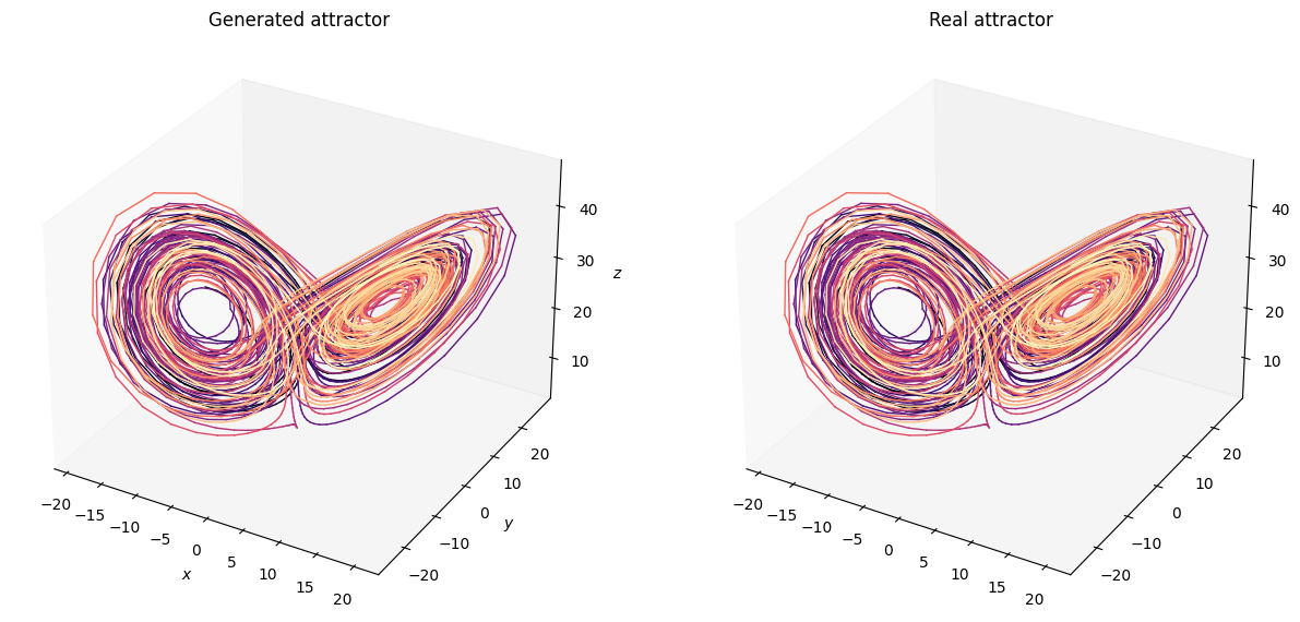
Despite its simplicity, it has been demonstrated in ^{7 1} that NGRC can consistently learn the flow of the Lorenz63 system, with and without the accessible inputs, therefore demonstrating itself as a good digital twin of the system.

Here we report our reproduced results of an NGRC digital twin for a Lorenz63 system with a signal applied to the inputs :

Model card

The NGRC model has been trained using the following NVAR hyperparameters:

• delay = 2 ; Maximum delay of inputs
• order = 2 ; Order of the non-linear monomials
• strides = 1 ; Strides between delayed inputs
• ridge = 2.5e-6 ; L2 regularization parameter

The output of the model is a vector of dimension 3 defined as

while the input is a vector of dimension 6 defined as The training data has been generated by numerically integrating the Lorenz63 set of equations using the RK23 method (Explicit Runge-Kutta method of order 3) with as initial conditions and . This means we discretize the system every 0.025 (in time units), where 0.025 is the discretization interval.

The warmup time chosen is 5 (in time units), dividing the warmup time by the discretization interval we find there are 5/0.025 = 200 data points for the warmup period. The training time is 50 (in time units) and the test time is 120 (in time units).

The design of this NGRC model can be easily generalised for creating a digital twin of another system if the conditions defined previously are met.

NGRC capabilities

When the data available for training are limited, they may not be sufficient to train the model. However, if some conditions are met, new researches suggest a new way to continue the training of the digital twin model and overcome this limitation. It is based on back-feeding the prediction of the digital twin and using them as training data in a sort of loop.

An interesting detail is that thanks to Taken’s embedding theorem, NGRC is also able to make inference about a hidden state of the system that is not observable.

Model-free NGRC controller

Before going into the details of the proposed approach is essential to review the main ideas it is based on ⁷.

System dynamic inversion

As stated above, the flow can be defined as follows

In general, this function is not invertible since there may be multiple possible input trajectories that drive the system to a given future state and not all states may be reachable from the current state. However, if we restrict the domain to future states reachable from the current state, we can effectively invert this function as

where is the function of interest for devising a controller for Eqs. 19 and 20 that choose a principle value among possible inputs.

NGRC controller

By focusing on the controller model in more detail, what we are trying to do is to create a model that learns to approximately invert the system’s internal dynamics by implicitly learning from data the inverted flow associated to the system. Then the x(t + δ) value is replaced with a desired future value obtaining a control action as output.

This has been proven possible and effective with Echo State Networks (ESN), a type of reservoir computing artificial neural network, as demonstrated in ⁷. One of our contributions is to use an NGRC model for the closed-loop controller. The NGRC controller will be designed as well as the ESN controller but with all the advantages over the classic reservoir computing models discussed earlier.

However, this function depends on the internal state , whereas only the observation is available to the controller. In a general scenario, this signal may be missing important information about , such as when projects onto a lower-dimensional space. Despite this, thanks to Taken’s embedding theorem, as stated above, the NGRC can infer the hidden states. We suggest that given the NGRC mathematical equivalent to a reservoir ANN then it is also able, under certain conditions and with enough data, to synchronize with its input ¹³. In other words, a reservoir coupled to and will tend towards some function of and . Accordingly,

The model

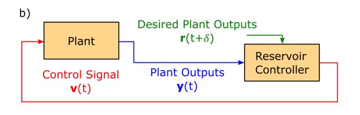
Initially, the system is stimulated with a signal that if appropriately generated is able to extract all the information needed to implicitly devise a control law. The result of the stimulation is saved associating to the stimulation vector the output induced.

At this point, we are able to construct 2 time series as follows:

where is discrete with discretization interval , and is the resultant vector from the concatenation of the vectors and .

The NGRC model is trained with the same setup and hyperparameters as the digital twin model. In input to the model we feed and as output we expect the model to predict the control signal applied to the system. Once the model is trained, in order to control the system, the is replaced with where is the desired reference signal we want the system to follow. By doing so, the predicted output is the control signal.

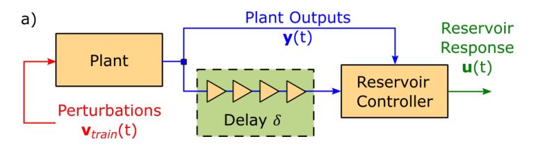
Finally, to start controlling the system, the controller must be inserted in closed-loop with the system as explained in the illustration below.

Nonetheless, even if effective, does not converge to 0 since the model only approximately learns . Clearly, for contexts where precise control is critical, an algorithm to improve the control error is necessary, in alternative avoiding this approach is strongly advised. Indeed, surprisingly, increasing the number of warm-up and training data points does not lead to a reduced control error, but it decreases .

Generating

Crafting an optimal stimulation signal is essential to obtain good model performance. Concerning this topic, it must be said that it is one of the most important problems in system identification. If the perturbation signal is poorly selected we may not be able to accurately identify the system or we may lose some particular behaviour of the system dynamics (for example at some frequencies). Although we can almost arbitrarily choose a signal a condition must hold. In particular, for eq. 21 to be verified must change slowly with respect to . Thus, must be bandwidth limited with frequency cutoff with . Concentrating on the crafting of the signal these guidelines are an effective yet simple way of finding a good control signal ⁷. Since frequency is already determined, it is also important to think about the magnitude . Generally, large perturbations will be easier to learn because they have a greater effect on the plant. However, this may not be the best way to learn to control the plant, and real-world control applications often require bounded inputs. Our approach is to generate a training signal from a uniform random distribution, which is Fourier-transformed, and frequencies above are dropped. The signal is then inverse-Fourier-transformed, and scaled to the range yielding with the required properties.

Digital twin backtesting/validation of the NGRC controller

Once a control law is devised, and the controller is working, a key issue is its validation, which is by itself a challenge. Directly testing the controller on the physical system can be harmful, damaging the components if something goes wrong. This may cost money and time and is not a very safe way to test a new controller. In addition, physically creating and making the controller operative may further increase costs and the time needed to test the solution.

For this reasons, we propose to completely virtualise a control system project after the initial data collection of the stimulated system. To simplify, what we suggest is to put the controller in closed-loop with the digital twin. For the test to be more robust, it is preferred to train the two models on different data points. Alternatively, the digital twin model may generate new data for training the controller, though if the digital twin does not model the system accurately enough the controller may not be able to control the real system while being able to control the digital twin.

In this way, it is possible to test the controller without any of the issues above. The strength of such an approach is that only with the initial data, and even with limited computational resources, we can design a controller for a system that exhibits chaotic behaviour, strong nonlinearities, and high complexity. Everything with ease and in a relatively short time.

In short, when precise control is not needed, this approach is not only effective but also efficient under every aspect.

Experimental results

We tested our approach against one of the hardest problems available, the Lorenz63 system. First of all, after demonstrating the NGRC digital twin capabilities, we created a model-free NGRC controller. We tested its capabilities in two ways, the first one was by inserting the controller in closed-loop and integrating numerically.

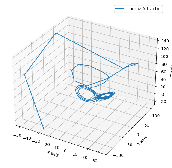
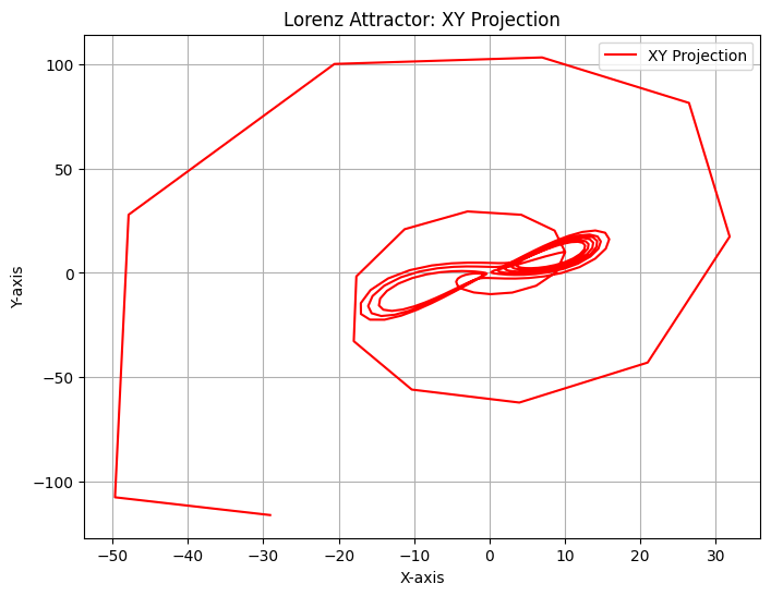
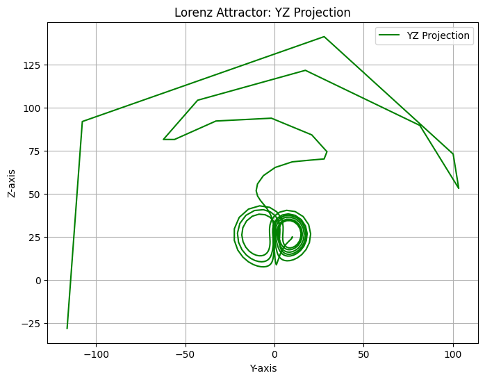
Here we plot, the evolution of each component of the Lorenz system when the controller is enabled. The objective of the control is to force the system to .

This is the 3D plot of the controlled system.

XY Projection

XZ Projection

YZ Projection

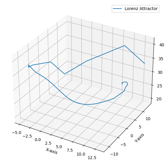
Then, we tested the model in a second way in closed-loop with the digital twin model.

Conclusions

In conclusion, our proposed method presents a novel approach to completely virtualize control system projects, enabling the creation and validation of controllers using a digital twin without prior knowledge of the plant (model-free). This method demonstrates promising results even in controlling systems exhibiting spatio-temporal complexity, nonlinearity, or chaotic behavior. Unlike other machine learning/deep learning methods capable of controlling systems of similar complexity, NGRC proves to be more efficient across various aspects while maintaining comparable performance. It requires less computational power, is sample efficient, and boasts faster training and execution times due to its mathematical simplicity. Moreover, NGRC offers a degree of interpretability, as the high-weighted nonlinear functionals can be traced back to the physical model of the system, thereby peeling back the ‘black box’ nature of many ML algorithms.

Moving forward, further exploration and experimentation are needed to rigorously validate and analyze the performance of the proposed methods. While this article provides a comprehensive discussion illustrating the potential applicability of our approach, it does so without any claim to mathematical rigour. Additionally, future research directions, such as the application of Hybrid-NGRC ¹⁴, may offer potential avenues for reducing control error, despite probable performance trade-offs due to the hybrid nature of such architectures.

Footnotes

1. Daniel J. Gauthier, Erik Bollt, Aaron Griffith, and Wendson A.S. Barbosa Next Generation Reservoir Computing ↩ ↩² ↩³ ↩⁴

2. Brian M. de Silva, Kathleen Champion, Markus Quade, Jean-Christophe Loiseau, J. Nathan Kutz, and Steven L. Brunton., (2020). PySINDy: A Python package for the sparse identification of nonlinear dynamical systems from data. Journal of Open Source Software, 5(49), 2104 ↩

3. Kaptanoglu et al., (2022). PySINDy: A comprehensive Python package for robust sparse system identification. Journal of Open Source Software, 7(69), 3994 ↩

4. M. W. Grieves, “Complex systems engineering: Theory and practice,” (American Institute of Aeronautics and Astronautics, Inc., 2019) Chap. Virtually Intelligent Product Systems: Digital and Physical Twins, pp. 175– 200 ↩

5. Daniel J. Gauthier, Ingo Fischer and André Röhm Learning unseen coexisting attractors ↩ ↩²

6. Lacerda et al., (2020). SysIdentPy: A Python package for System Identification using NARMAX models. Journal of Open Source Software, 5(54), 2384 ↩

7. Daniel Canaday, Andrew Pomerance, Daniel J. Gauthier Model-Free Control of Dynamical Systems with Deep Reservoir Computing ↩ ↩² ↩³ ↩⁴ ↩⁵ ↩⁶

8. D. Gauthier, “Reservoir computing: harnessing a universal dynamical system,” 51:2, 12 (2018). ↩

9. Gonon, L. & Ortega, J. P. Reservoir Computing Universality with Stochastic Inputs. IEEE Trans. Neural Networks Learn. Syst. 31, 100–112 (2020). ↩

10. Hart, A. G., Hook, J. L. & Dawes, J. H. P. Echo State Networks trained by Tikhonov least squares are L2(μ) approximators of ergodic dynamical systems. Phys. D Nonlinear Phenom. 421, 132882 (2021). ↩

11. Bollt, E. On explaining the surprising success of reservoir computing forecaster of chaos? The universal machine learning dynamical system with contrast to VAR and DMD. Chaos 31, 013108 (2021) ↩

12. F. Takens, “Detecting strange attractors in turbulence,” in Dynamical systems and turbulence, Warwick 1980. Springer, 1981, pp. 366–381. ↩ ↩²

13. Z. Lu, B. R. Hunt, and E. Ott, “Attractor reconstruction by machine learning,” Chaos, vol. 28, p. 061104, 2018. ↩

14. Hybrid Reservoir Computing to Forecast Complex Dynamics (Dael Amzalag - TREND REU 2023) ↩