The central limit theorem, together with the law of large numbers, is one of the most fascinating theorems of statistics. Their applications range from economics to biology and therefore are popular and known among scientists. However, I found that it’s very common to forget the hypothesis behind them and apply them even when they does not work. Or better, to apply them where they may work on paper but not in the real world. This is mainly due to the oversimplification in reminding the theorems. For instance, regarding the central limit theorem, many people just remember that the sum of every distribution gets to the normal distribution. Well, this is, of course, true but the rate at which the distribution of the averages converges to the true mean changes a lot depending on the initial distribution type.

Table of contents

• The Central Limit Theorem
  • Theorem
    • Explanation
  • What does this mean to us?
  • Where is the problem?
  • What can we bring home from this?

The Central Limit Theorem

First of all, let’s review the formal definition of the Central Limit Theorem (from now on called CLT). It is important to note that there are different variants of the CLT but we’ll refer to the Lindeberg–Lévy’s one.

Theorem

Given sets of random samples from a population, where each sample set has finite mean and bounded variance . Then as approaches infinity, the random variable converge in a normal distribution with and .

Explanation

The classical central limit theorem describes the size and the distributional form of the stochastic fluctuations around the deterministic number  during this convergence.

More precisely, it states that as  gets larger, the distribution of the difference between the sample average  and its limit , when multiplied by the factor  — that is,  — approaches the normal distribution with mean  and variance . For large enough , the distribution of  gets arbitrarily close to the normal distribution with mean  and variance .

The usefulness of the theorem is that the distribution of  approaches normality regardless of the shape of the distribution of the individual .

What does this mean to us?

Translating the mathematical formulas into jargon, less clean, but more clear while at the same time comprehensive, it says this:

The distribution of the means of groups of random samples, with any distribution shape, of a population is normal with . In particular, by the law of large numbers, the mean of the distribution of the means converges to the population mean.

Extra: Other variants of the CLT require additional conditions like Lyapunov’s one that asks for independence between the random variables but not that they are identically distributed. If a sequence of random variables satisfies Lyapunov’s condition, then it also satisfies Lindeberg’s condition. The converse implication, however, does not hold.

Where is the problem?

Plainly speaking, CLT is used in a lot of contexts to handle a distribution that differs from a normal like a normal. Because, as some remind it: “All distributions end up being Gaussian”. This is useful but it can be misused very easily. Indeed while on paper it works in reality it doesn’t, and this is why.

While for most distribution shapes CLT converges for , this doesn’t hold for fat-tailed distributions or power-law distributions. (Here we should define what is a fat-tailed distribution in a more formal way… but this isn’t really the point so we’ll skip it.)

Now we’ll demonstrate it through numerical tests.

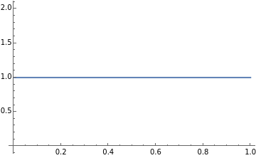
Let’s start using a uniform distribution between 0 and 1

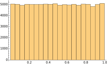
At this point, let’s sample times from the uniform distribution This is the underlying distribution of the samples:

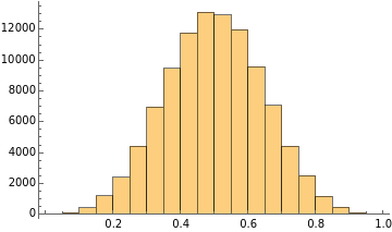
Here things start to get interesting. If we sample 2 elements and sum them up times the associated distribution looks like this

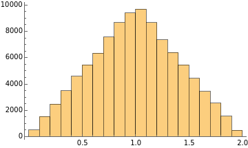
As you can see, the distribution is already not flat. The most likely probability is at 1 because to get 1 there are a lot of combinations, while to get 0 or 2 you need a lot of work because only 0 can give you 0, and only 2 can give you 2.

CLT is already working, if you sum numbers or average numbers you end up with a Gaussian. The problem is that this example reaches the central limit very quickly. But this is not always the case.

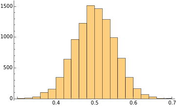
For those who don’t believe until they see, here it’s the distribution of the averages. We start creating sample sets, each of dimension 4, sampling from the uniform distribution and the distribution of the averages of the sample sets is this:

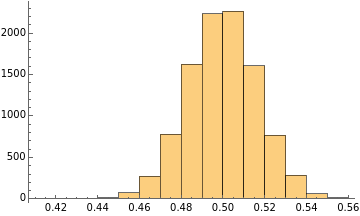
I want to make a little digression here to fully understand how the central limit theorem works in practice. From now on, we’ll work on the averages of the sample sets. Specifically, this digression will focus on how the final distribution changes its shape depending on the dimension of each sample set. We note an interesting behavior that can be summarised as follows:

As the dimension of each sample set increases, the final distribution has lower variance around the mean.

This is due to the law of large numbers, in fact, as the dimension of each sample set grows, the mean of the sample set will tend to the true mean better and better.

Sample size: 30 Number of sample sets:

Sample size: 300 Number of sample sets:

Until now, everything worked as expected… Let’s try to break it. We’ll use a Pareto distribution. The Pareto distribution is a power-law distribution. For those interested in the technical details, here is the formal definition:

And this is the distribution shape:

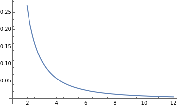
In this example, we’ll use a Pareto distribution with shape parameter () of 1.14 and scale parameter () of 1.

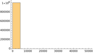
Now let’s do the same we have done before but this time using the Pareto distribution. This is the result with a sample size of 30 and sample sets:

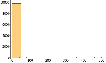
This result might seem unexpected, but it’s not an error. As everybody can see, the distribution significantly deviates from a Gaussian shape. No matter how you look at it. If you understand why this happens then you may say: “Let’s increase the number of sample sets”. In fact, the theorem states “when goes to infinity”. So let’s try with sample sets:

Still no bell shape on the horizon. We could continue increasing the number of sample sets, but we stop here because to get a bell shape, with a sample size of 30, you need sample sets. That is a very economical number, for those who understand what I mean.

However, no matter how you see this, it has a lot of implications. If you are using CLT in the real world on a fat-tailed distribution you will be dead way before your model starts to work.

To help you grasp how big is I’ll just say that seconds are about 316 887 years.

What can we bring home from this?

Well, there are two different reasons this happens:

• First of all, the Pareto distribution with has infinite variance and CLT requires bounded variance.

But while this is true, the Pareto distribution actually obeys the condition of bounded mean of the Law of Large Numbers.

• This means that (and this is also due to the infinite variance) despite it being bounded, the mean jumps around a lot.

This means that to compress the variance and to get the mean with the same reliability as a non-fat-tailed distribution you need a lot more work.

All this work brings us to the conclusion that when working with fat-tailed distributions, applying the CLT to know the mean may not be a good idea (here I’m ironically optimistic). Actually, looking for the mean may not be a good idea at all because, for a fat-tailed distribution, it is not a very robust property.